Simulating a car suspension system
on an EAI 580 analog computer

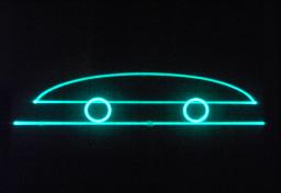
A few weeks ago I became the very proud owner of a wonderful EAI 580 analog computer which was given to me by the Institut für Meß- und Regeltechnik of the University of Karlsruhe (I would especially like to thank Mr. Böhringer for his help and support).

After cleaning the system and repairing some minor faults (currently only four of the 64 operational amplifiers are still defective and only one double integrator has problems with its control circuitry) I was looking for a suitable problem to solve using this wonderful machine. Since its integrators employ electronic switches for mode control and since the machine has quite a few electronic switches which can be used to form analog multiplexers for example, I decided to reimplement the vehicle simulation I did on the Telefunken RA 741 analog computer without any special external equipment like my four channel oscilloscope multiplexer.

The picture below shows a screen shot of a running simulation. The model consists of the road on the bottom which is excited by a variable frequency sine generator with variable amplitude, a set of wheels which are simulated in detail including their spring constants and, finally, the frame of the car which is mounted to the wheels by a pair of springs and dampers which are also taken into account in this simulation. (Clicking on the picture will download a 1:47 minute video showing an actual simulation - this video file is about 8.5 MB in size!)

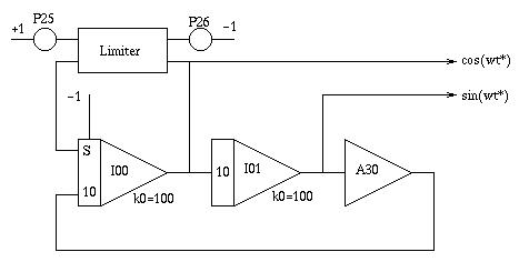
Some of the mathematical background of this simulation may be found on the page describing my other vehicle simulation and in great detail in the "Handbook of Analog Computation" (pp. 91) published by EAI in 1967. In the following only the completed circuits and potentiometer settings are shown.

As nearly always when graphical output is desired, a high frequency (several kHz) sine-/cosine-generator is needed which output signals will be used as the basis for all figures to be displayed. The circuitry for this basic generator is shown below (in fact it simply solves the differential equation y''=-y) - normally one would employ a positive feedback for one of the integrators to avoid a decaying output signal. It turned out that the integrators of the EAI 580 tend to increase their output signal over time when running in high speed mode (2 ms integration time constant) so only a limiter is necessary to avoid overloading the integrators).

The two output signals of the circuit shown below will be used throughout the rest of the simulation circuits described here.

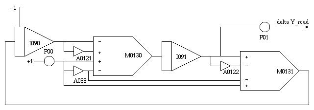
While the old vehicle simulation used a noise generator with a low frequency filter I decided to employ a more deterministic way of road simulation for this project. Here a variable low frequency generator will be used - its circuit is shown below. Essentially it works exactly like any other sine-/cosine-generator but the inputs of the integrators are preceded by two parabola multipliers driven in lockstep with a signal ranging from 0 to +1 thus effectively affecting the frequency of the output signal.

Using P00, a handset coefficient potentiometer, the frequency can be set while P01 allows to change the amplitude of the road displacement.

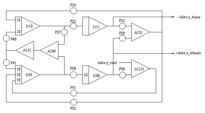
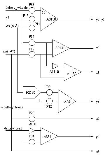
Using the road displacement output signal of the circuit shown above it is now possible to feed it into the simulation of a simple two mass system containing springs and dampers. The complete circuit for this part of the overall simulation is shown here:

Putting all together we now have a high frequency sine/cosine signal pair as well as y-displacement signals for the road, the wheel set and the car frame. These displacement signals now have to be added to the high frequency signals to generate the impression of moving figures on the display of an oscilloscope. This is done with the following sub-circuit (the function generator F2120 is used to create a somewhat car-like figure):

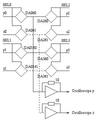
Now we have four coordinate signal pairs (y0, x0), ..., (y3, x3) for the wheels, the car frame and the road accordingly. To display all of these four figures at once on an oscilloscope some multiplexing has to be done. Fortunately, the EAI 580 features some digitally controlled analog switches which can be grouped together to form a four channel multiplexer. Using the circuit shown below the four separate figures are displayed in rapid succession on the screen of the oscilloscope thus creating the impression of a car on a road.

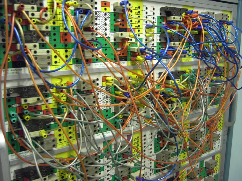
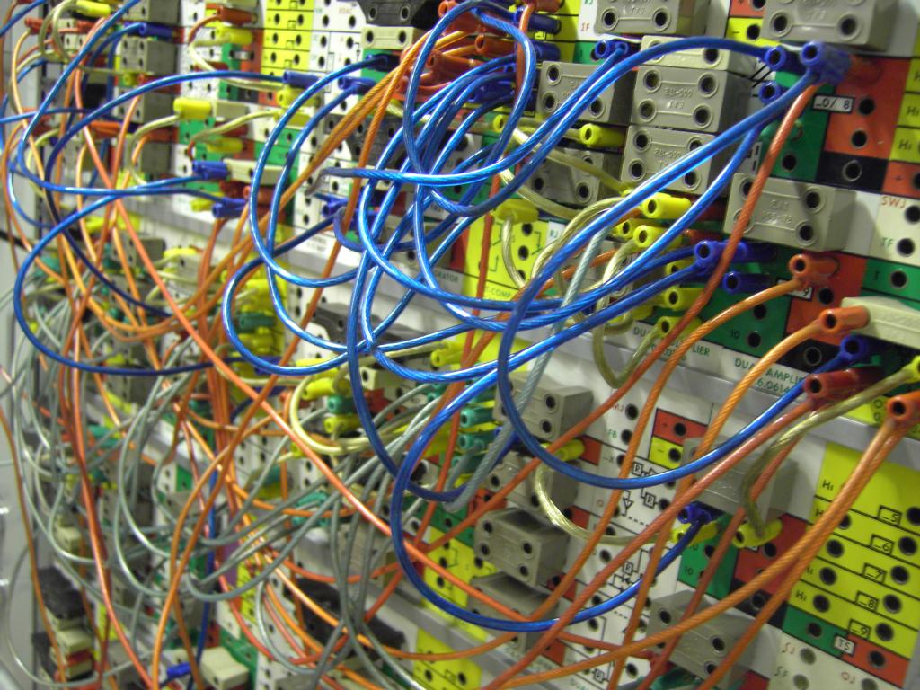
The following two pictures give an impression of the overall setup of the analog part of the simulation. As can be seen this problem uses not quite half of the computing elements of the EAI 580 analog computer.

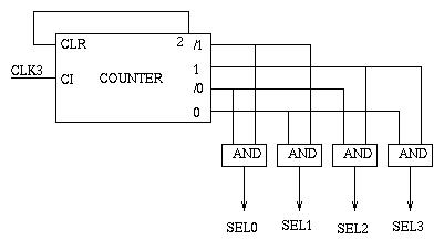
What is left now is a means to generate the digital control signals SEL0, SEL1, SEL2 and SEL3 used in conjunction with the muliplexer circuit shown above. Generating these signals is fairly easy - I just use a binary counter counting from 0 to 3 and decode its normal and inverted output signals to generate the four selection signals. The actual circuit generating SEL0 to SEL2 is shown below:

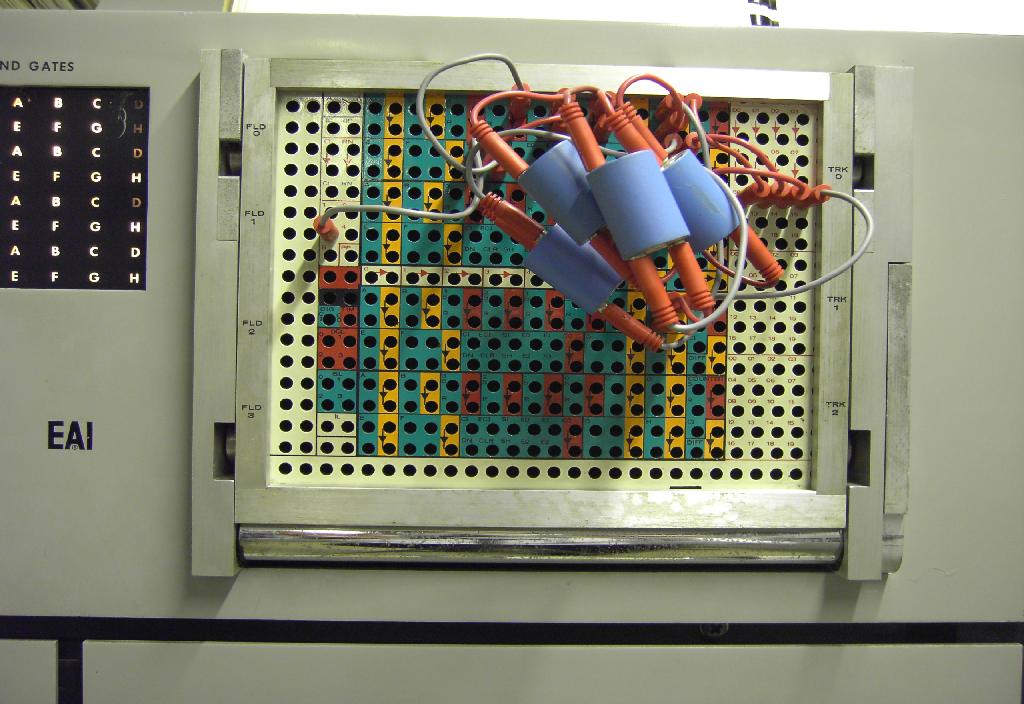
The picture on the right gives an impression of the digital setup of this simulation. Due to the small size of the digital patch panel of the EAI 580 the circuit described above looks quite crowded although it is really simple. The cylindrical objects are so called free multiples - just metal blocks with holes to create connections between two or more cables.

The overall simulation makes use of 23 coefficient potentiometers which are listed with their appropriate values in the following:

The main control parameters are set using P24, P28, P31, P32, P40 and P41. Due to the optimized two mass simulation circuit shown above these coefficients are lumped parameters, i.e. they depend on more than one problem variable.

The short video clip was, for example, created using the following main parameter settings:

Using these parameters yields the following settings for the central control potentiometers:

Of course the values used to derive these potentiometer settings are far from being realistic, but I wanted to show the overall behaviour of such a two mass system rather than design a real car suspension system (which, of course, would be quite possible using this setup with proper parameters).

The picture on the left shows the complete setup of this simulation. On the top right of the EAI 580 analog computer the oscilloscope used to display the car running on the road can be seen.

I hope you enjoyed this simulation and the circuits descriptions. If you have questions or suggestions, please let my know (see mail address below). Happy analog computing! :-)