| How to simulate a ball bouncing in a box |
|
| How to simulate a ball bouncing in a box |
|
|
|
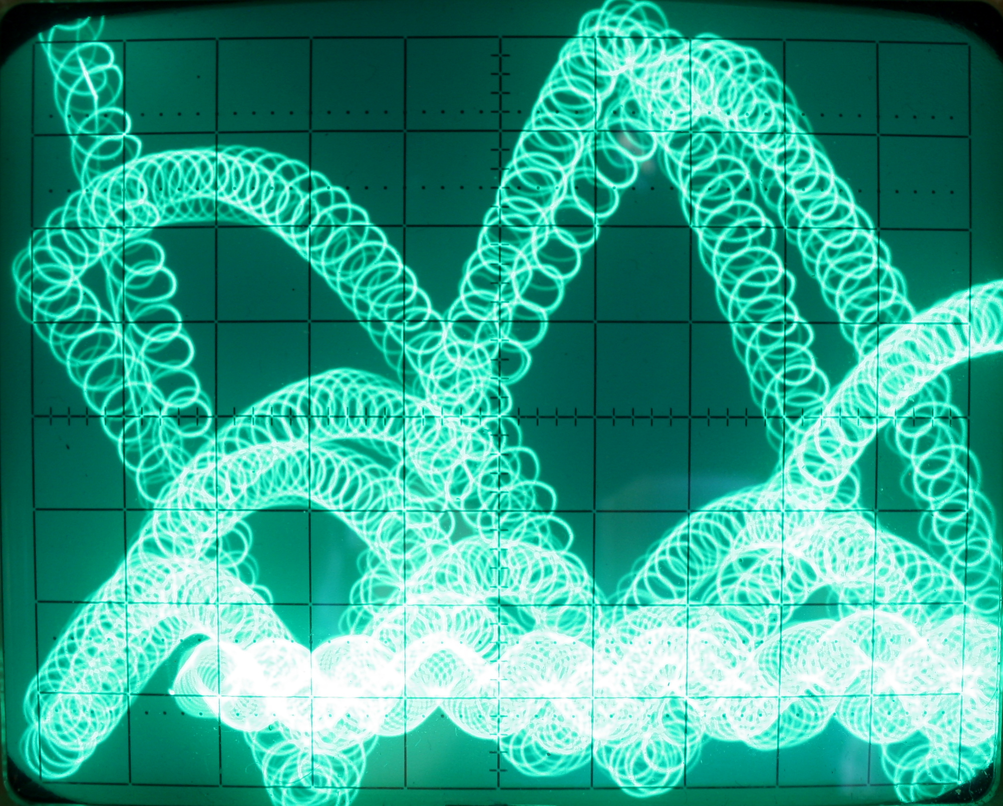
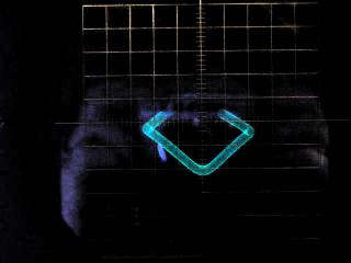
About 40 years ago TELEFUNKEN published a short paper with a description of the simulation of a bouncing ball in a box (a scan of the original paper may be found here). The basic idea is fairly simple - all in all three different circuits solving some differential equations are used. One circuit calculates the y-position, another circuit calculates the x-position of the ball while the third circuit generates a high frequent sine/cosine-pair which is superimposed over the x- and y-values to generate a round ball. The picture above shows a long time photograph of a simulation run taken by Tore S. Bekkedal during the VCFE 2007 where I displayed this simulation. |
|
|
Calculating the y-position of the ball in the box: The circuit below shows the generation of the y-position of the ball. Potentiometer 1 determines the gravity which acts upon the ball. Potentiometers 5 and 10 are used to set the initial values for the velocity (P5) and y-position (P10). Potentiometer 2 is used to set the damping value - the higher it is set the faster the ball will loose its energy through the elastic rebounce. The two Z-diodes are part of a simple trick: The original TELEFUNKEN circuit used two open amplifiers to implement a dead zone to create an upper and a lower limit of the box where the ball will be reflected. Due to a severe lack of free diodes, I decided to implement a box of height -1...+1 which is the task of the two diodes (which, in fact, are just four 4V7 Z-diodes). 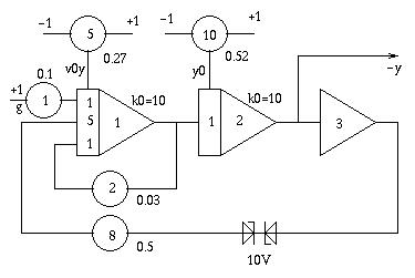
|
|
|
Calculating the x-position of the ball in the box: Calculating the x-position of the ball is a bit more tricky and involves two comparators (which make a wonderful small "click" sound whenever the ball hits one of the two walls). Integrator 14 gets an input signal which absolute value starts at 1 and runs towards zero, so the ball looses speed while bouncing in its box. The comparators are used to change the sign of the input signal of integrator 14 every time the ball hits a wall to change its current direction and reflect it from the wall. 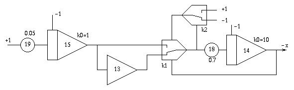
|
|
|
Making a real ball: The picture below shows the circuit generating the sine/cosine-pair to create a real "ball" on the oscilloscope screen. It simply solves the differential equation y''=-y thus generating a sine and a cosine. Please note that the integrators are fed at their junction points thus making no use of the integrator resistor input networks. These are replace by two free potentiometers 11 and 16 which allows the generation of a high frequency signal. In addition to this the time constant k0 is selected to be the highest possible on the analog computer used (an RA742). Potentiometers 11 and 16 can be used to change the frequency of the generated sine/cosine-pair. Potentiometers 12 and 13 determine the diameter of the ball (elliptic balls are thus possible, too). Potentiometer 4 is necessary to stabilize the circuit. 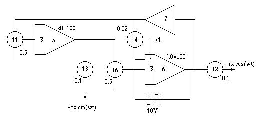
|
|
|
Putting it all together: |
|

|
The circuit on the left shows how to mix all of the output signals of the preceeding subcircuits in a manner to generate proper x- and y-signals for the display oscilloscope. Two amplifiers with unity gain are used to superimpose the sine/cosine-signal with the raw position signals -x and -y as generated before. |
|
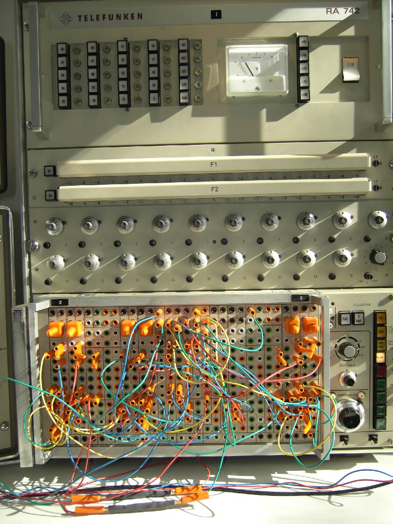
The picture on the right shows the overall setup of the program to simulate a bouncing ball in a box. The two thin, black things in the foreground are the two +-10V Z-diodes used to limit the ball in its y-direction and to limit the high frequency sine/cosine-generator. Since integrator 15 will eventually hit its limit and this causing an overload stop of the computer it proved useful to run the program in repetitive mode. The time constant of repetition has been selected in a way that ensures that the input of integrator 14 will reach nearly zero causing the ball to stop. Another advantage of this setup is the fact that the computer can control the brightness of the display oscilloscope which has no automatic x-deflection and is quite sensitve to burn in of the electron beam. |
|
|
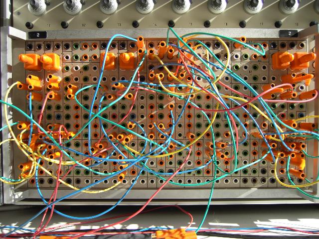
The picture below left shows the patch panel in more detail - try to match it with the circuit diagrams above. :-) The picture on the right will lead to an AVI-file of the bouncing ball (caution this file has a size of about 6 MB so download will take a moment!). |
|
|
|
| 24-FEB-2006, 26-JAN-2008 |