|
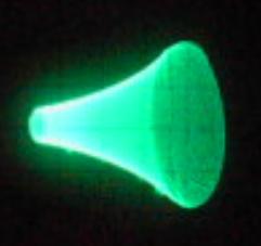
The following page shows how an analog computer can be put into use to display a three dimensional figure on an oscilloscope in real time allowing for interactive changes of parameters during the computation run. The picture below is a screen shot from the oscilloscope's display - clicking on the picture will load an AVI-movie (about 3.3 MB). In this movie it can be seen that it is possible to influence a running computation on an analog computer on the fly by adjusting the coefficient potentiometers which is done while the figure is moving in space as well as with a steady figure. |
|
|
|
|
One of the most fascinating properties of an (electronic) analog computer is the fact that such a machine is not only capable of solving (complicated) differential equations in real time. In addition to that an analog computer is a highly interactive device allowing the operator to immediately experience the effect of parameter changes during a running program. Last weekend I decided to setup a small program to display a three dimensional figure on an oscilloscope. The figure on display should be rotated around one axis showing all side of it during a run. This requires a so called repetitive computation: One part of the program will generate the outline of the three dimensional figure over and over again in rapid succession to create the impression of a steady figure on the display, while the other part of the program will generate the necessary sine- and cosine-values for the rotation of the body. Since both parts of the program involve integrators it is necessary to control two groups of integrators independently of each other - one is working constantly in run mode to generate the rather slowly changing sine-/cosine-signals, while the other one is switched in rapid succession between initial-condition and run. This requires an explicit integrator control program which is implemented on a digital expansion unit of the analog computer used (this program has been implemented on my EAI 580 system which was donated by the Lehrstuhl für Meß- und Regeltechnik of the University of Karlsruhe and will be described in way more detail soon on these pages - I would like to thank Mr. Böhringer and Prof. Stiller from the faculty for this donation). The following sections describe the overall program which was used in the generation of the movie shown above. |
|
|
Generating a pair of sine-/cosine-signals: Generating a coupled pair of sine-/cosine-values using an analog computer is simple - is merely involves solving a differential equation of the general form y=-y''. The corresponding circuit is shown below and consists of two integrators and two summers used as sign inverters (the second summer is necessary since the actual rotation will be performed using two quarter square multipliers).
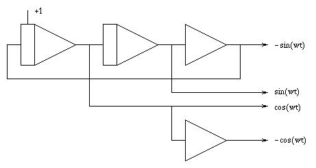
This part of the program will be initialized once and then continues to run while the part described in the following will run in the repetitive mode described above. |
|
|
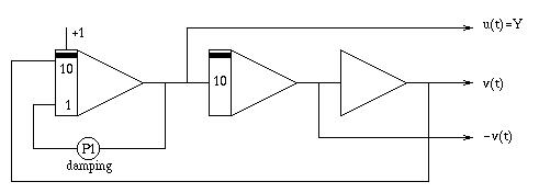
Generating a three dimensional figure: To generate a three dimensional figure it is necessary to generate a coordinate tripel for every point of the hull of the figure. For this example I decided to use a simple spiral linearly stretched in a third dimension. The circuit below generates the X and Y coordinates of a basic spiral - the program is nearly identical to the one above which was used to generate the sine-/cosine-signal pair. The main difference is that the spiral program contains a damping parameter which degrades the circle which would evolve without damping to a spiral. The output value u(t) will be used for the Y-deflection of the display while v(t) will be used in conjunction with the sine-/cosine-signal pair generated above and the third coordinate as shown below. Changing the value of the coefficient potentiometer P1 shown below will change the steepness of the spiral on display. Since this circuit has to generate a spiral in rapid succession its integrators are not controlled by the normal control of the analog computer which is denoted by the black bars in the upper half of the left hand side of each integrator figure. The necessary control signals will be generated with a circuit shown below.
|
|
|
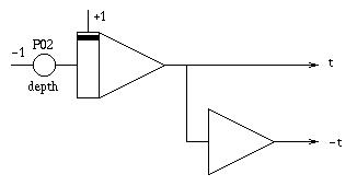
Adding the third dimension: Transforming this flat spiral into the hull of a three dimensional body can easily accomplished by using a linearly increasing variable like the machine time as the necessary third dimension. This variable is generated in repetitive mode, too, using the circuit shown below:
|
|
|
Putting it all together: |
|
|
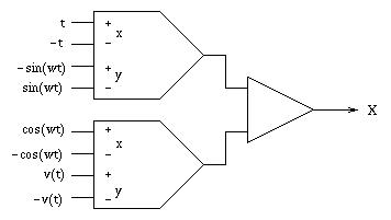
Mapping this figure described by the three coordinate values u(t), v(t) and t itself to a two dimensional display is now fairly easy. All that is necessary is a sine-/cosine-value pair and two multipliers followed by a summer as shown in the figure below:
|
|
|
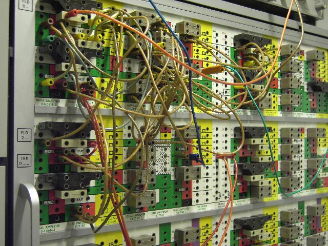
The pictures on the left shows the overall program setup for the analog part of the simulation - as you can see only a small fraction of the patch panel is occupied by this program. |
|
Controlling the repetitive integrator group: As already described above it is necessary to control the group of three integrators for generating u(t), v(t) and t independently from the rest of the computer to create the impression of a steady picture. This is done using some digital elements to create the two standard control signals used by an electronic integrator: RUN and IC (initial condition) - the halt mode is not used here. The circuit shown below consists of a single AND gate used as an inverter and driver and two decade counters to generate the necessary pulse sequence to control the three integrators. The signal denoted CLK2 is generated by the analog computer's control circuitry and has a frequency of 100 Hz:
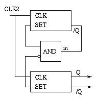
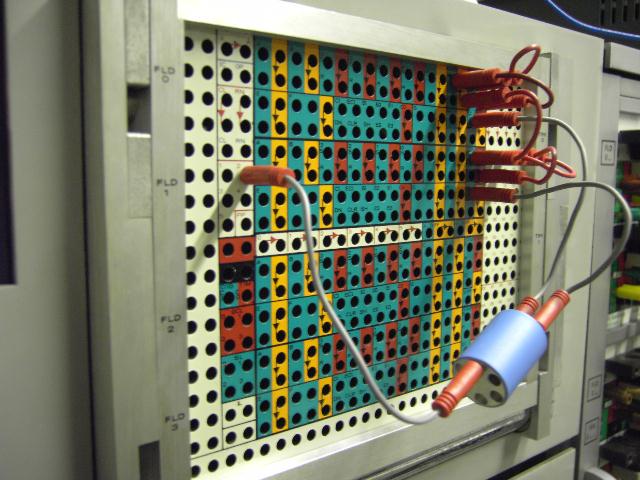
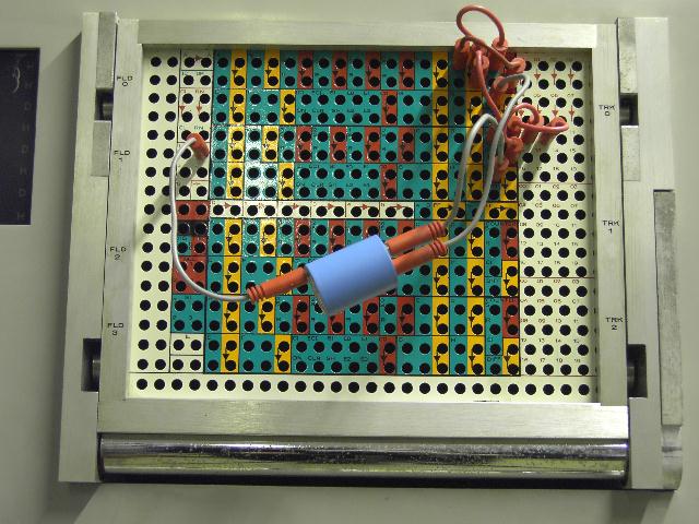
Q is used as IC signal while its inverse, /Q, serves as the RUN signal for this integrator group. Please note the the AND-gate shown has a single input and two outputs - one normal and one inversed which are used to preset the counters. The output Q of such a counter will stay true until a predetermined number of clock inputs has occured. The two pictures below show the digital control program. On the left of the patch board the signal CLK2 can be found while the counters and the single AND-gate used are on the far right. The connection to the analog patch panel shown above is implemented using prewired trunk lines so easy access to the signals generated here is possible from the analog portion of the program. |
|
|
|
|
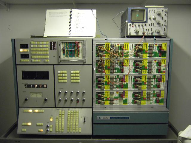
The picture on the right shows the overall setup of the program. The analog computer used is, as already mentioned, a wonderful EAI-580 hybrid electronic analog computer. The right hand side contains the analog computing elements located behind the patch panel while the left hand side contains the control electronics, the digital voltmeter and the digital expansion chassis. On top of the machine sits a Philips oscilloscope which was used to make the movie which may be found at the top of this page. |
|
|
I hope you enjoyed this demonstration of the power of (electronic) analog computing. If you have questions or know of an analog computer which needs a good home, please feel free to contact me. All the best and happy analog computing - Bernd. :-) |
|