A very simple orbital rendezvous simulation

I have always been very interested in the early days of space flight when the USA made their first steps into space with their Mercury and later Gemini programs. One thing of particular interest to me was and still is the technique of orbital rendezvous between two space ships - establishing these techniques was one of the goals of the Gemini program.

When you think about space dynamics (by the way - there is a wonderful book repulished by Dover: "Introduction to Space Dynamics" by William Tyrell Thomson which makes a very good reading and is way more affordable than the (great) book by Krafft-Ehricke) it becomes clear quite quickly that docking two space craft together in an orbit is not that simple at all.

Even considering two coplanar and circular orbits, as will be done in the following, the fact that orbits with smaller radii will yield higher angular velocities than orbits with larger radii, makes catching up another space ship quite counterintuitive.

I have thought for quite a while about doing a simple rendezvous simulation to get a feeling for the mechanics of space flight, so I did not attempt a very accurate simulation. This yields to some (over-) simplifications as well as some clear errors: The orbits of both space ships are thought to be coplanar and being perfectly circular. Moreover the function yielding angular velocity from orbit radius is just inversely linear yielding smaller angular velocity for larger radii and vice versa.

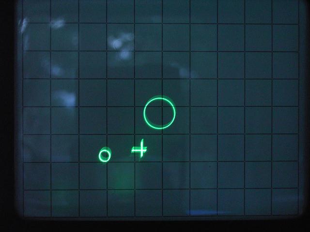
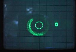
The picture on the left shows a snapshot of the simulation - in the middle is the earth, the target is denoted by a cross while the maneuverable space ship is denoted by a small circle (this display uses my four channel oscilloscope multiplexer).

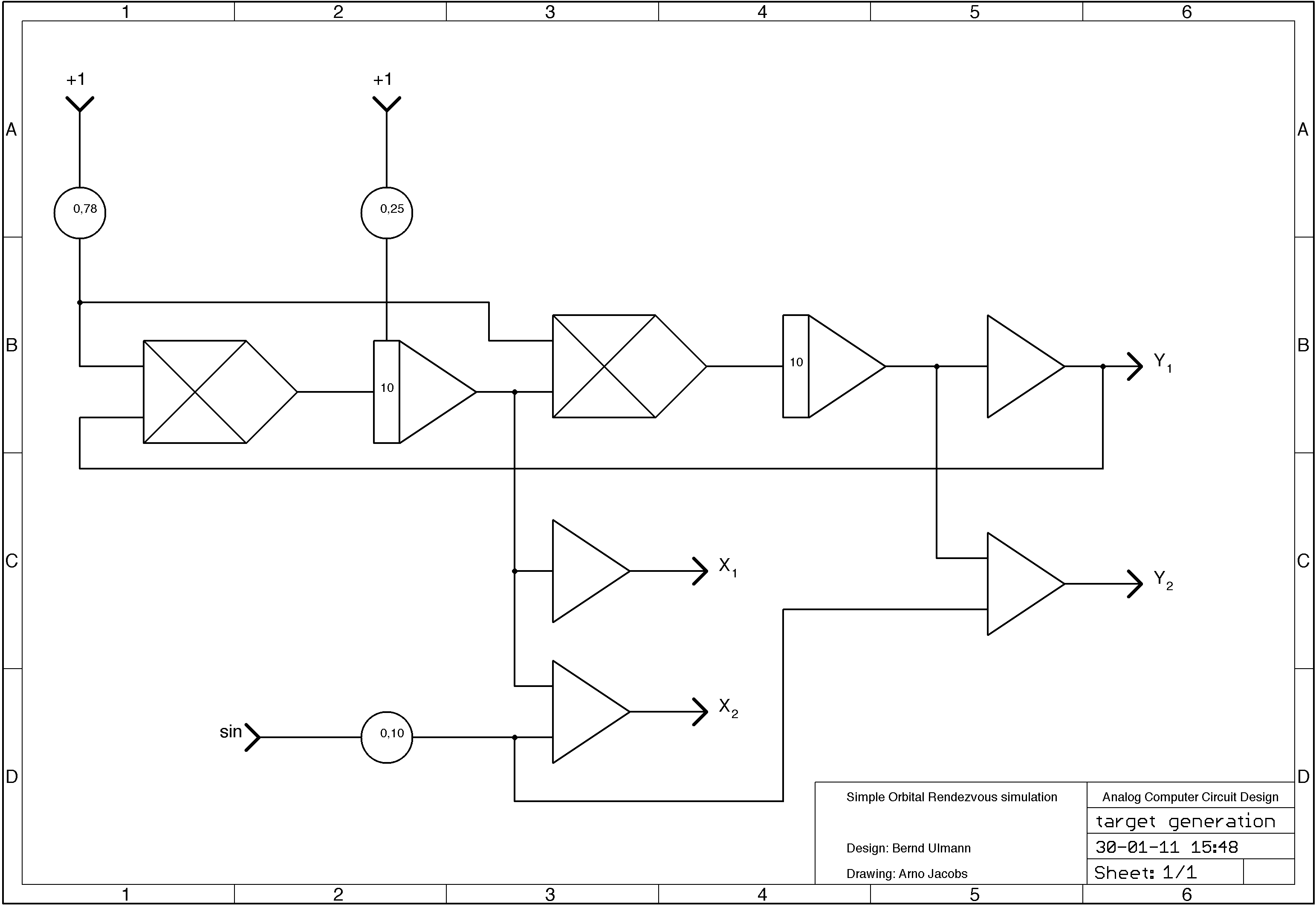
First of all we need a target orbiting around the earth on a simple circular path. This is done using the analog program shown on the right, which just solves a differential equation of the form y''=-y while the frequency of the solution may be set using two multipliers (I would like to thank Arno Jacobs for his wonderful circuit drawings).

To generate the cross (and the circle of the earth and the space ship described later) a pair of high frequency (about 500 Hz) sine-/cosine-signals is needed - these may be generated using a circuit similar to that of the target generation but with higher frequency. In this setup I use a home brew quadrature generator to save two integrators, a summer and two potentiometers since I often need such a signal pair in my programs.

Since the target is displayed as a cross, it requires to X/Y-channels of the four channel oscilloscope - the raw target coordinates are summed with the high frequency sine-/cosine-signals respectively giving one horizontal and one vertical bar moving in an orbit around the simulated earth (which is just a plain pair of these sine-/cosine-signals).

Generating the space ship is a little bit more difficult than generating the target since the target runs in a fixed orbit while the space ship can change its orbit (all the time being circular and coplanar to the target orbit.

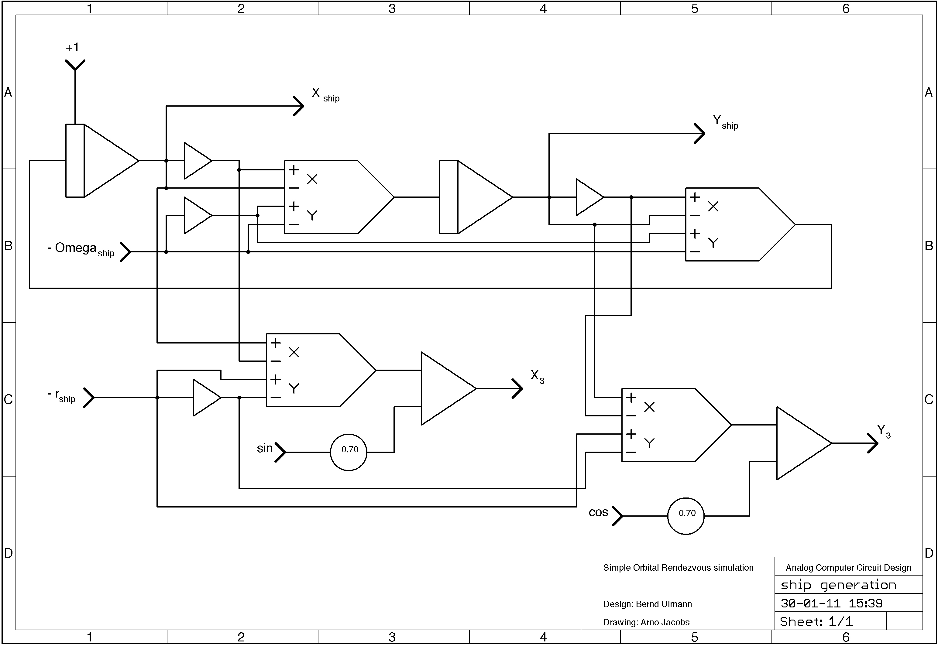
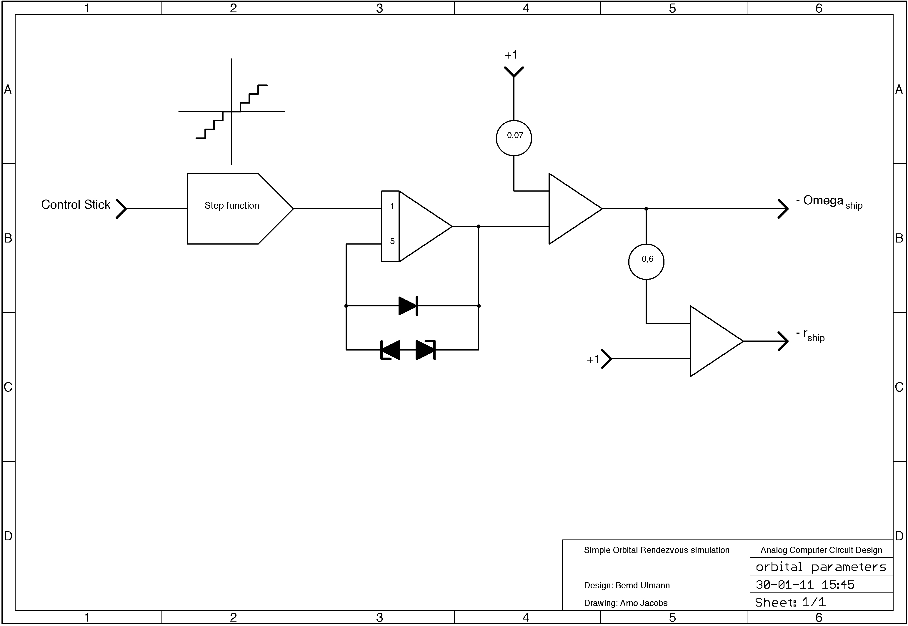
The circuit on the left shows the generation of the ship - the two multipliers forming a loop with two integrators just solve something like the well known y''=-y with varying frequency (giving a varying angular velocity of the ship) while the two multipliers on the bottom determine the orbit radius.

To steer the space ship I assume there is a reaction control system allowing for generating thrust in the direction of flight or in the opposite direction. The thrusters are controlled using a single axis of my homebrew control stick. Since such thrusters normally have no linear thrust control, the output of the control stick is fed into a function generator set to generate a step output function allowing for two different levels of thrust in each of the two basic directions thus slowing the space ship down or speeding it up (this directly controls the angular velocity and the radius of the orbit).

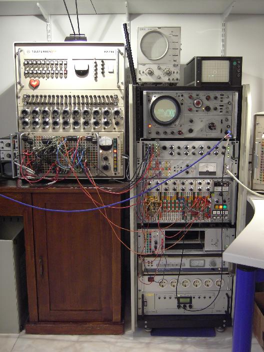
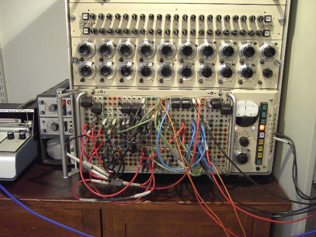
The picture on the left shows the overall setup of the ship generation and the calculation of angular velocity and orbit radius depending on the levels of thrust controlled by the "pilot". This part of the simulation occupies most of a Telefunken RA 741 table top analog computer.

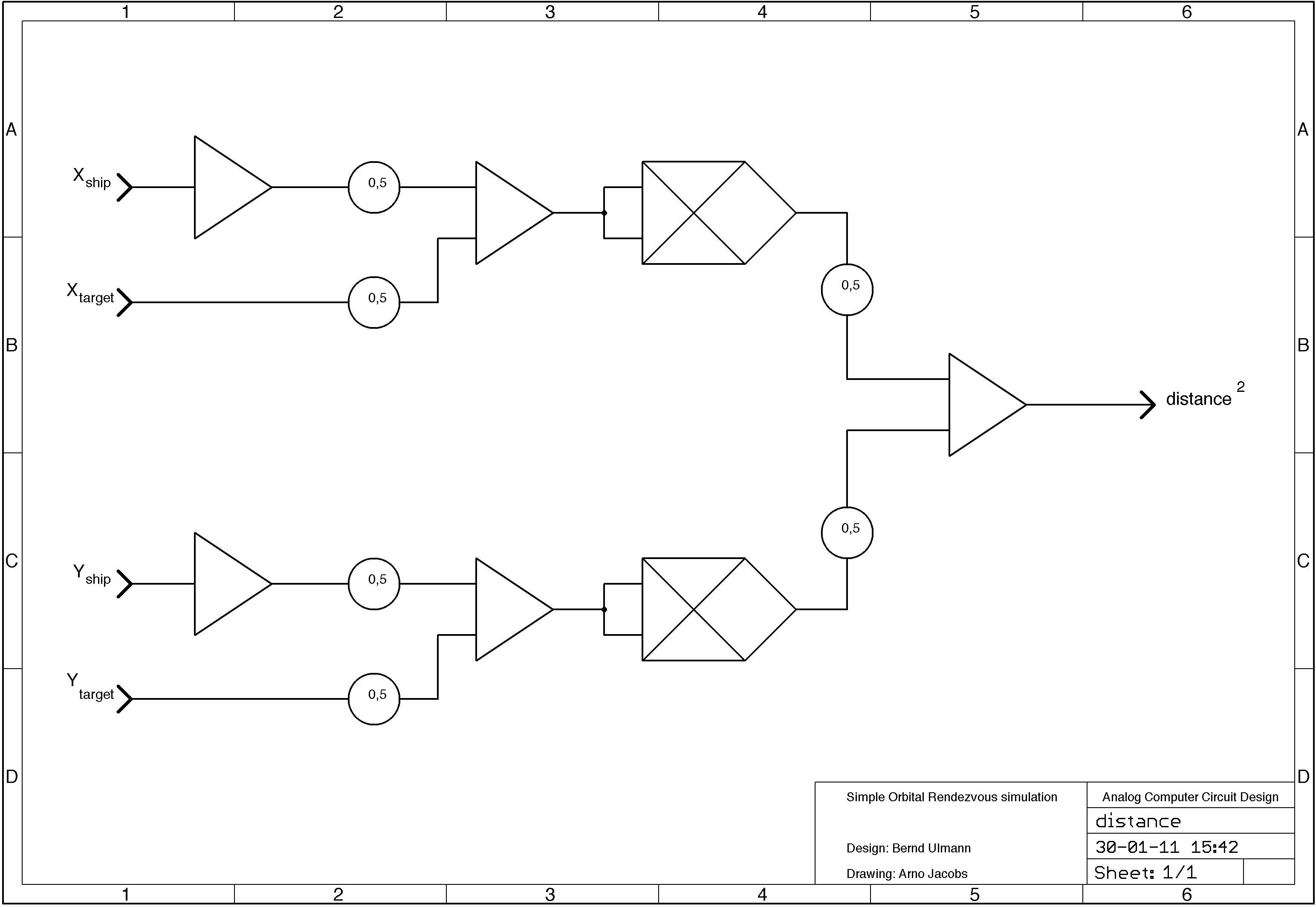
Given the cartesian coordinates of the target and the space ship it is easy to calculate the distance between the two using the euclidean norm with a circuit like the one shown on the right. The output of this circuit is the square of the distance - unfortunately I had no multiplier left to calculate the square root so the distance output is squared.

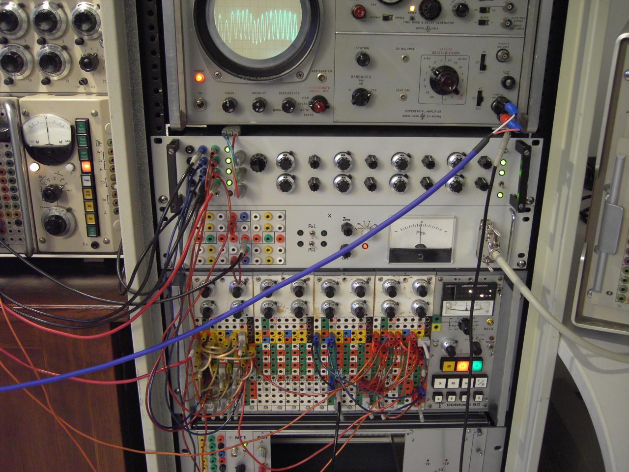
The picture on the left shows the setup for target generation and distance calculation. On top of the rack part of a HP storage oscilloscope can be seen. Below is the four channel oscilloscope multiplexer and the control stick assembly. On the bottom a small Dornier DO-80 analog computer can be seen which is used for these calculations.

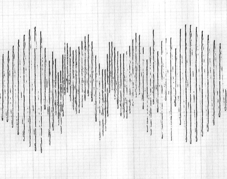
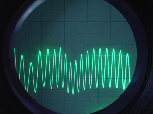
The two pictures below show two records of space ship/target distance (squared) - the picture on the left is the output of a simple x/t-plotter while the picture on the right was recorded with the HP storage oscilloscope shown above.

To get an impression of the simulation (at high speed - a more realistic simulation would run way slower but would be way more boring in a short video clip like this) can be seen by clicking on the picture on the right. This will download a 9 MB AVI file showing some seconds of the running simulation. Please note that the angular velocity on the maximum orbital radius of the space ship is very unrealistic, but the overall setup indeed gives a good feeling for the behaviour of space dynamics involving two space craft.

13-JAN-2008, ulmann@analogmuseum.org