|
Electronic analog computers were the backbone of the incredible developments in aerospace technology in the 1950s and 1960s - without their help progress would have been much slower if not impossible at all. There is a wonderful book Black Magic and Gremlins: Analog Flight Simulations at NASA's Flight Research Center that is not only fun to read but also very informative and addictive! :-) I was long since wondering how they did it - how does a purely analog flight simulator actually work? Imagine a 6 DOF aircraft simulation with all the necessary coordinate system transformations and rotations, with the vastly different domains for variables, with all the problems introduced by drift and noise during long simulation runs... This really sounds like one of the ultimate challenges and thus I HAVE to know. :-) Frederic found a great video clip on Youtube showing some footage of X 15 tests - the most interesting part, of course :-), is the simulator setup that can be seen from 00:00:38 until 00:01:01 (I would love to see what it shown on the monitor mounted on top of the cockpit). Comparing this footage with the pictures and text in "Black Magic and Gremlins..." there were a couple of EAI 231R analog computers driving this simulation. You can watch this part of the video clip below: 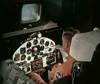
A couple of days ago my friend Frederic Fournis suggested starting with a very simple simulation:
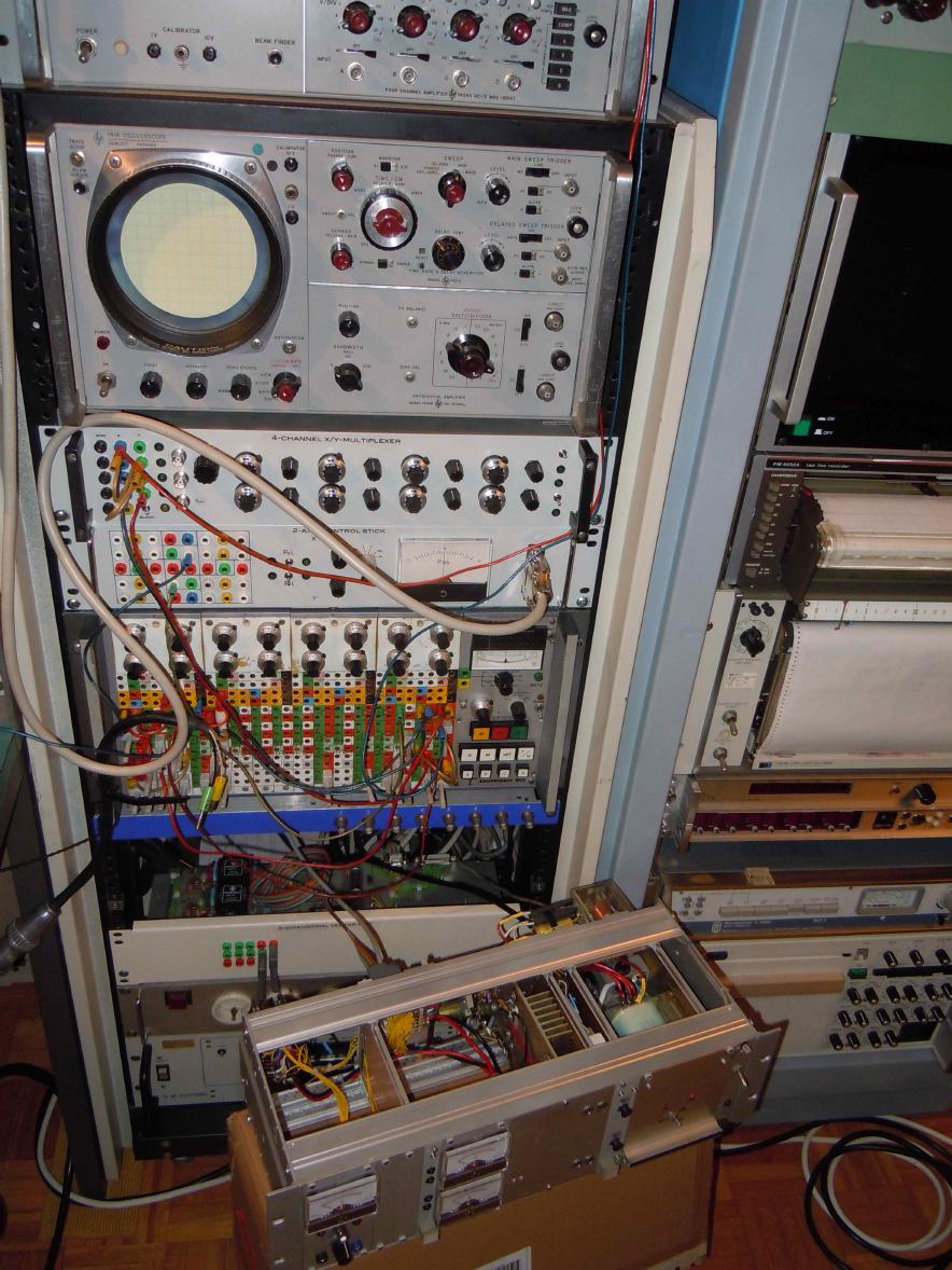
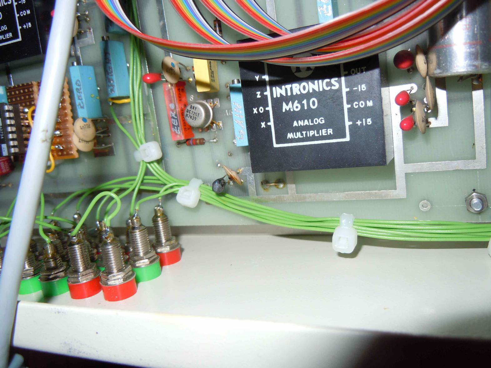
So how does one start? Have a look at the literature first. One of the analog "bibles" is the "Computer Handbook" by Huskey and Korn which also contains a short chapter about the basics of analog flight simulation written by Louis Bauer ("Aircraft, Autopilot and Missile Problems", in "Computer Handbook" by Huskey & Korn, 1962, pp. 5-51 ff.). In addition to that the book "Introduction to Electronic Analogue Computers" by C. A. A. Wass (Pergamon Press Ltd., 1955) has a short chapter dealing with a simple longitudinal flight simulation as the one I wanted to implement. Since I can think best with the analog computer running, so I can try out ideas at an instant, the first thing to do is to switch it on... Believe it or not, but the Gremlins have found their way not only from the 1960s into 2011 but also to the small village I live in - I was greeted with a hushed puff and a small white cloud of smoke followed by a nasty smell. Is that crazy? My machines are running flawlessly since years or at least months and the very first day I actually plan to implement a flight simulation something starts burning. What I really dislike when it comes to problems like this one is that it a) stinks and b) I fear that the damage might spread when I keep power applied for too long. So the process of searching with a flash light and my nose in the innards of one of the racks started. The two pictures below show the search for the Gremlin - the picture on the right side shows the little critter: A tantalum capacitor that was incinerated and caused the +15V power supply line to be shorted to ground (although the power supply managed to deliver about +9V :-) ). |
|
|
|
|
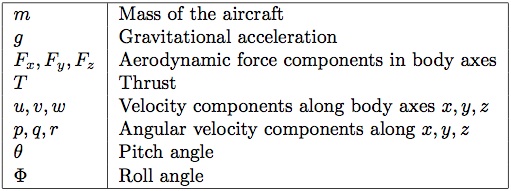
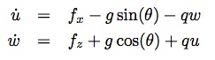
After fixing this problem, I started with actually thinking about the longitudinal flight simulation. First of all there are three dynamic equations describing the translation of the aircraft: 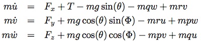
What is still missing is the elevator which is not to be found in the equations above. Therefore we need another equation describing the momenta around the y-body axis of the aircraft: 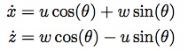
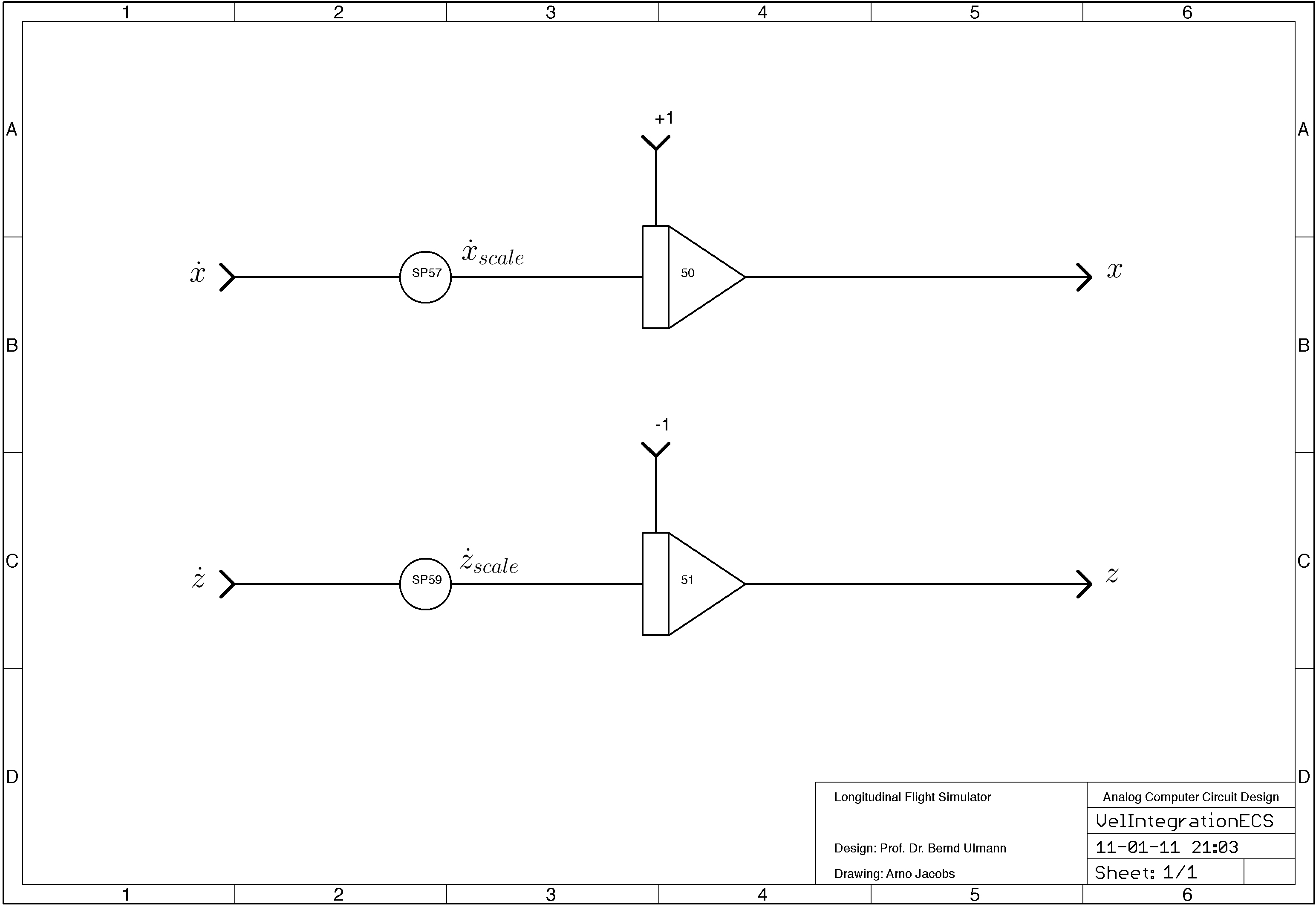
That's all - isn't that great? :-) Just kidding - it took me some time to figure that out and what I have concealed from you are the normalized coefficients of the simulation - these are really hard to determine due to the non linear nature of the DEQ system. To be honest, I do not have a good coefficient set at the moment - the simulation runs but with fantasy coefficients which ensure that no parameter will exceed the limits of +/-1 machine unit, but this is far from being a realistic simulation of a real (simplified) aircraft, so there is a lot of work to be done in the near future. Nevertheless this set of equations is enough to setup the computer and to start a simple simulation with (more of less cleverly) guessed parameters. The following schematics show the computer setup (they were drawn by Arno Jacobs who developed an Eagle CAD library with all the symbols necessary to draw analog computer setups - terrific! I would like to thank him very much for his support!) that was used for this 1st flight simulation. |
|
|
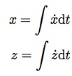
The picture on the right shows the circuit to implement the momentum equation yielding q and -theta (after an additional integration). The only input to the simulation is the free potentiometer on the left side of the picture which allows one to enter any elevator angle between +1 and -1. |
|
|
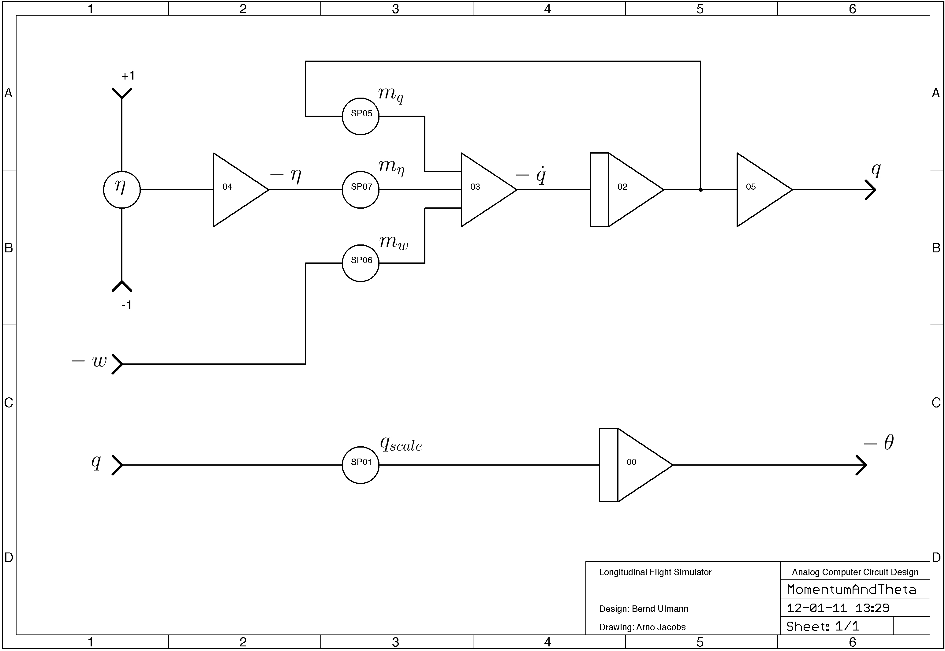
The picture on the left shows the circuitry to derive the necessary sine-/cosine-terms as well as the implementation of the acceleration equation along the body x axis. |
|
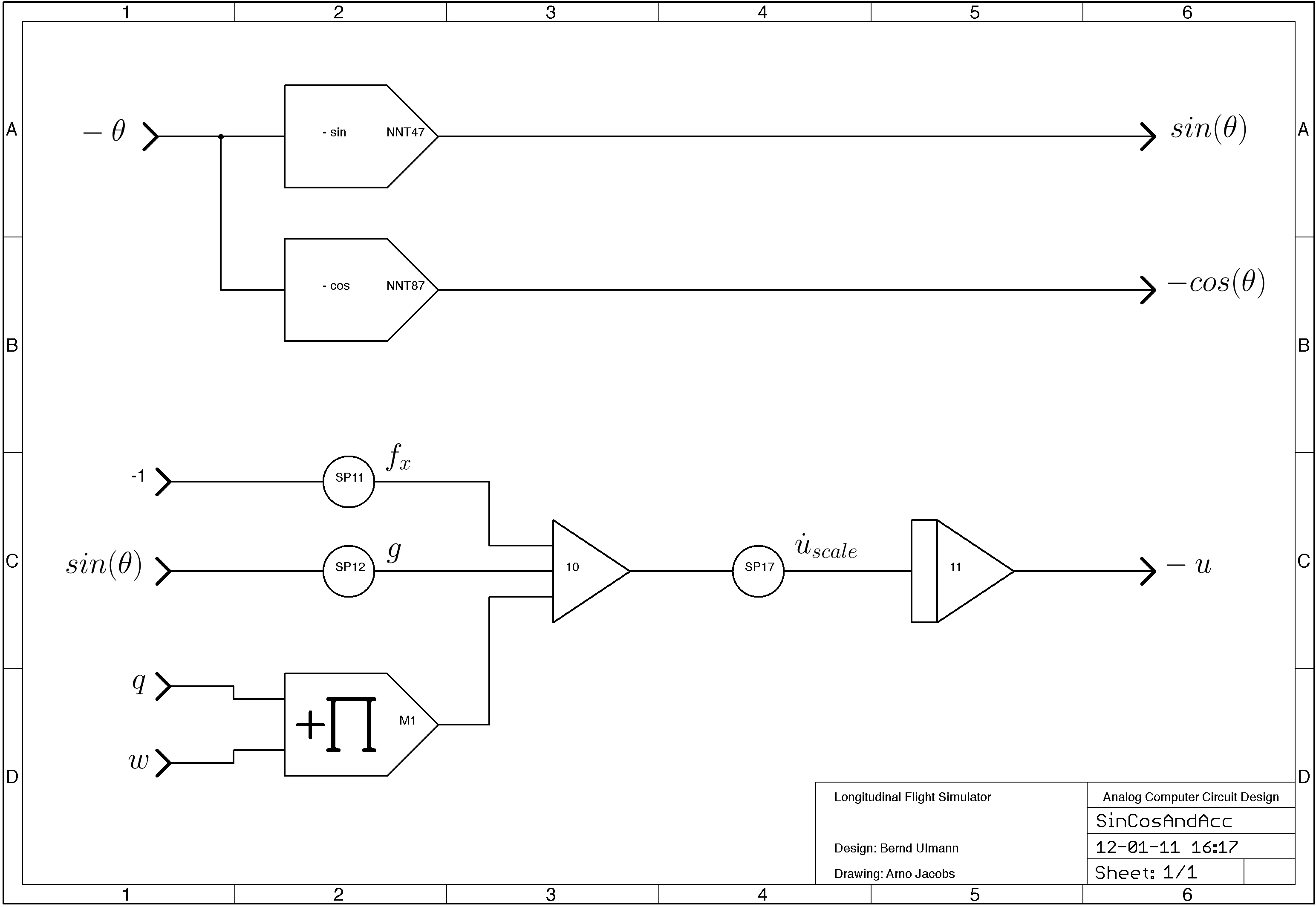
The circuit for the term w, the velocity along the body z axis is shown on the right: |
|
|
|
Given -u, w and the sine-/cosine-terms the circuit shown on the left transforms these velocities from body coordinates into earth coordinates. |
|
These velocities in ECS are then integrated (with a suitable scale factor to avoid running against the machine unit limit too soon during a simulation run) to yield absolute coordinates in ECS as shown on the right. |
|
|
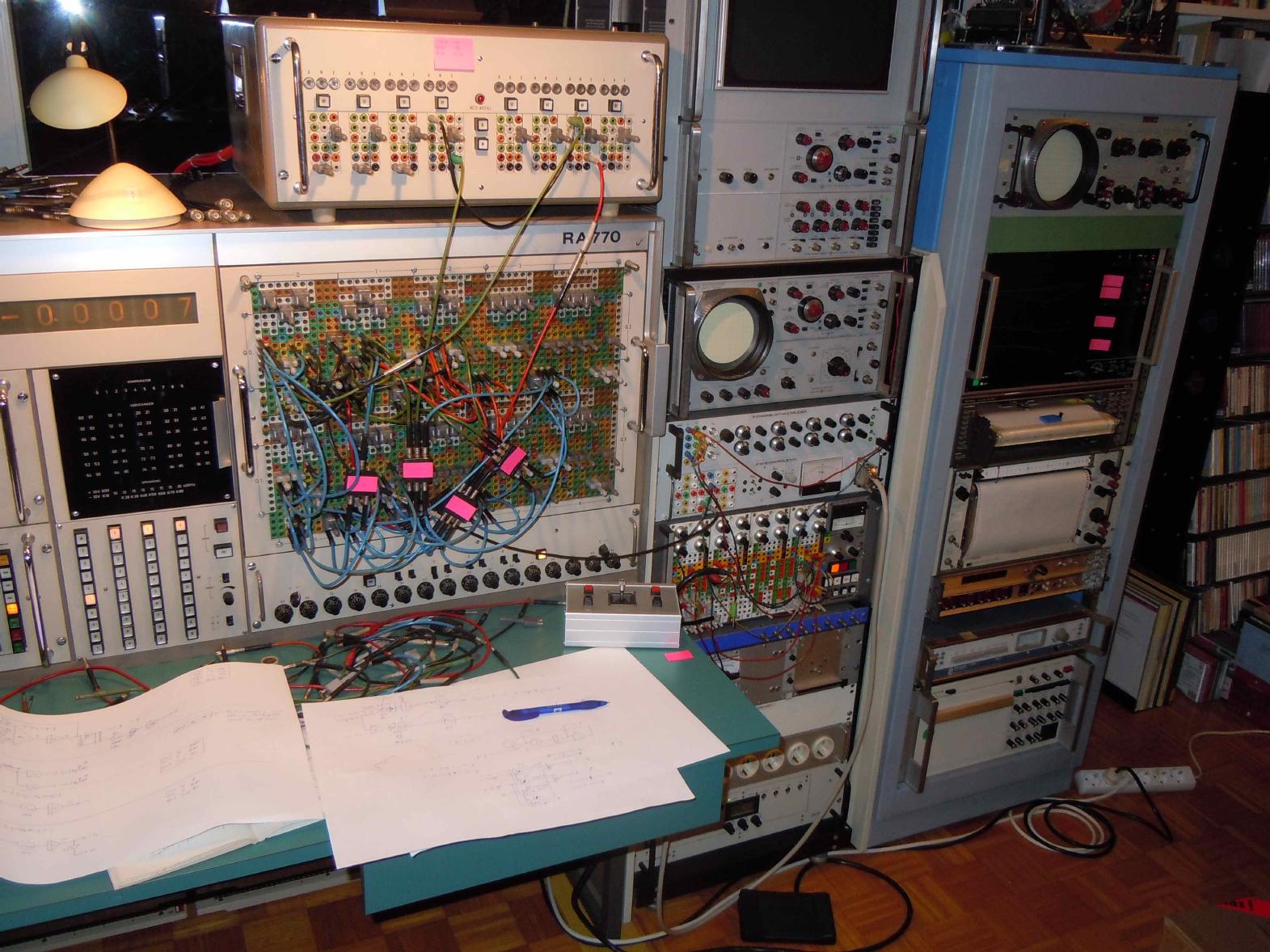
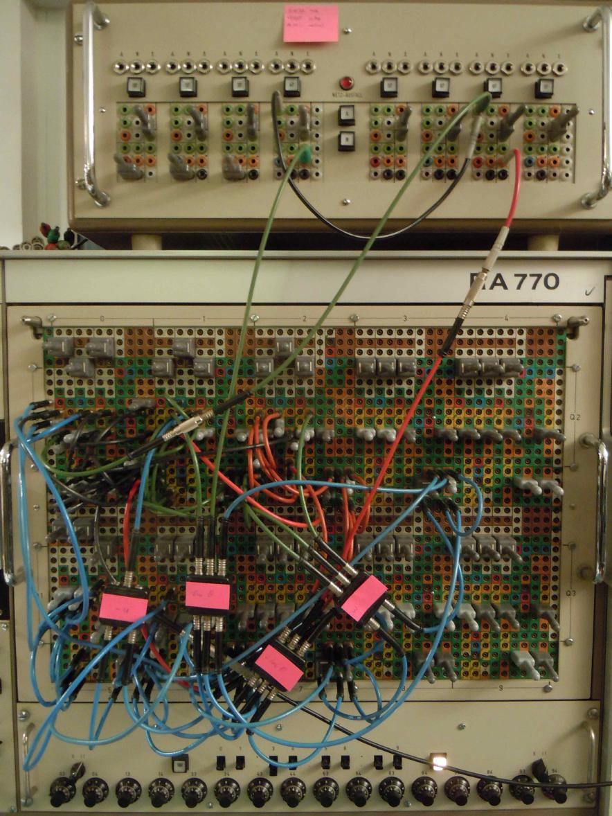
The picture on the left shows the completed analog computer setup on my Telefunken RA 770 precision analog computer. The unit on top of the patch field is a drawer containing non-linear elements - in this case it houses (from left to right) three multipliers, three sine functions and two cosine functions of which only one sine and one cosine are needed for this simulation. |
|
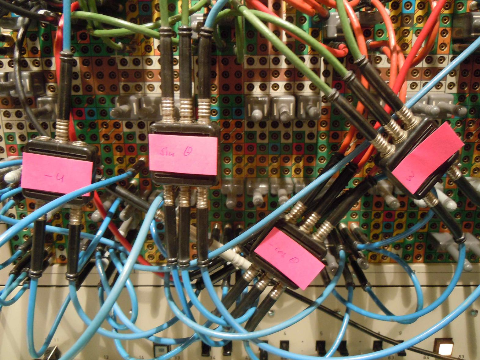
To avoid getting confused during setting up this simulation some adhesive markers were necessary to flag four of the most needed signals in the overall circuit as can be seen on the right. :-) |
|
|
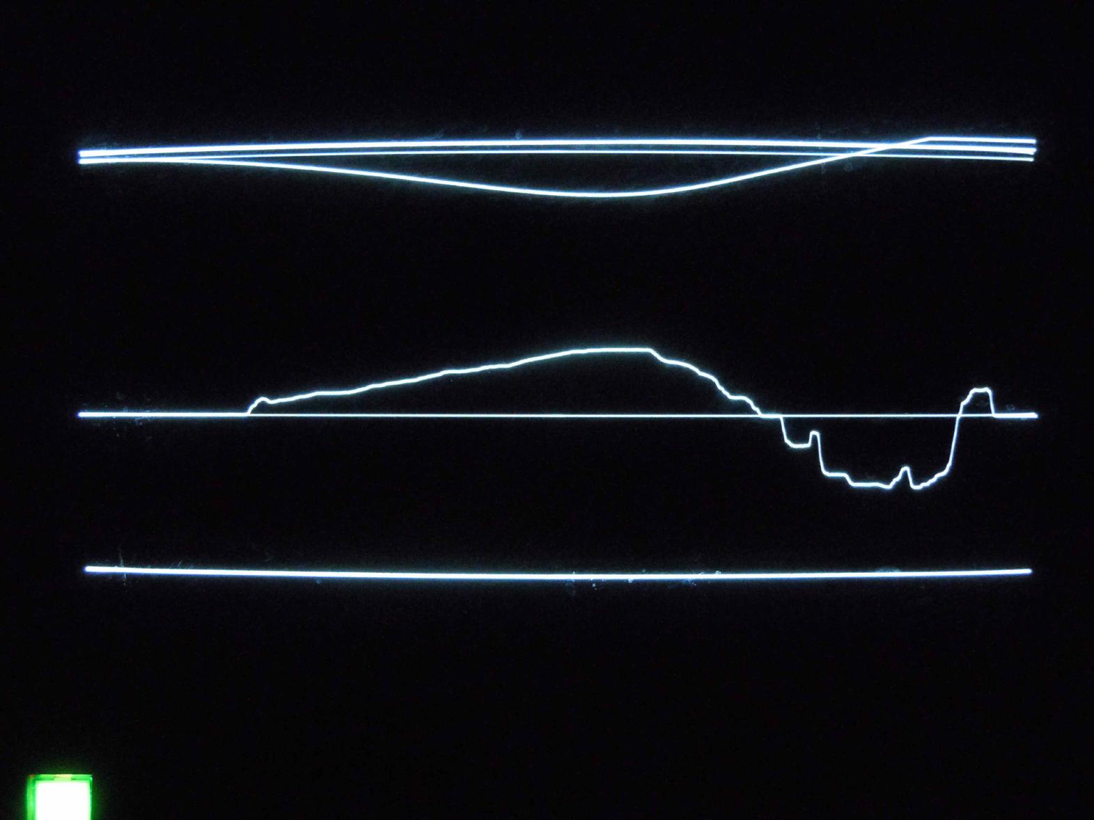
The picture on the left shows the first test run of the simulation (OK, not the first one, but the first one that behaved as expected - after I fixed a couple of sign errors and the like and found a set of coefficients that allowed at least a couple of seconds of simulated flight) - the top trace is the x coordinate of the aircraft in ECS - it barely moves from its zero line which is due to a too small scaling factor, but I wasn't that interested in x, so I did not change it for this run. More interesting is the second trace from top which shows the height of the aircraft. After being "dropped" the airplane starts to - hmmm - drop like a stone which I tried to compensate by moving the elevator. The wiggly line below shows the elevator angle eta as read from my homebrew control stick. As one can see the airplane reacts very slowly and I overshoot. After stopping the fall I can not compensate the climb and the z integrator overflows. But the simulation works (sort of). The next step will now be to derive reasonable coefficients to model a realistic (simplified) aircraft. |
|
08-JAN-2011, ulmann@analogmuseum.org |
|