|
On July 19th, 2008, my friend Dr. Matthias Koch brought a small mathematical problem to my birthday party: Suppose you are driving a car with an initial speed of 100 km/h. You are continuously loosing speed while driving - to be exact, you loose 1 km/h for every kilometer you drove. The question now is, how long does it take to drive 50 km with this style of driving? The first observation is that dv / ds = -1 since the graph of your speed plotted against the distance is linear, beginning with v = 100 km/h at s = 0 km and ending with v = 0 km/h at s = 100 km. Of course, you will never reach the point s = 100 km, but this is not the problem here since we are interested in the time it takes to reach a distance of 50 km. Thinking about the graph resulting from plotting the speed versus time it is obvious that v(t) must be of the form exp(-t) since the speed at any distance s is exactly 100 - s. Since the distance traveled at any time t is just the time integral over v(t) which is of the form 100 * exp(-x), one could write 
As nice as an this analytical solution is, it would (of course) be nicer to have a model of the problem on an analog computer to confirm the result obtained above. All we need is a computer setup for this problem. Assuming a scaled model where 100 km are represented by a machine value of 1, we can write v(t) = 1 - s(t), where s(t) is the time integral over v(t). The resulting computer setup is extremely simple: 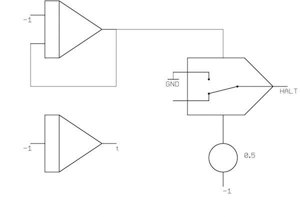
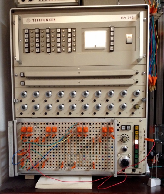
The lower integrator just yields the time integral over the constant -1. Its output directly corresponds to the time spent traveling. (By the way, the analog computer used is a Telefunken RA 742.)

The time required to reach 50 km is then computed as 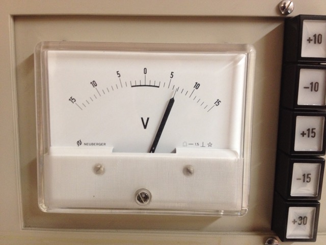
|
|
|
20-JUl-2008, 21-DEC-2008, 19-FEB-2016, ulmann@analogmuseum.org |